Predicted observed graphs
All models included in the APSIM release need to have validation tests built using the user interface. Graphs with observed data need to be created in a .apsimx file.
Observed data
Observed data needs to be in a spreadsheet (only .xlsx files are supported).
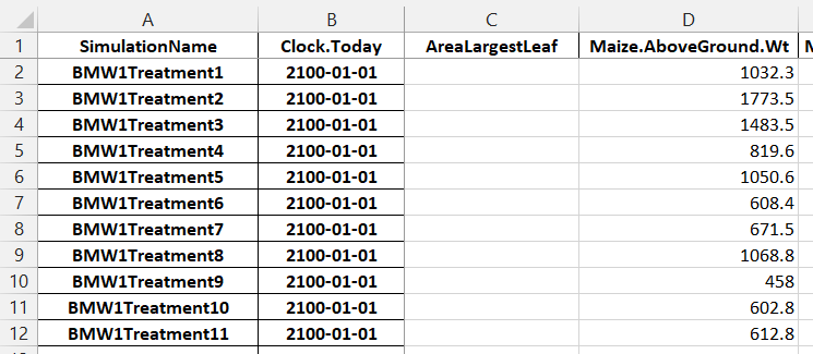
Observed spreadsheets must have a ‘SimulationName’ column with values that exactly matches the name of the simulations in the simulation tree. The column names also need to exactly match the column names in APSIM.
Multiple sheets can exist in the spreadsheet file. To connect the APSIM User Interface to the spreadsheet, an Excel component should be dropped onto the DataStore component, renamed to Observed and configured.
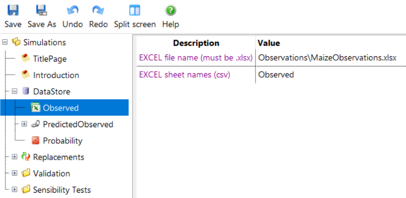
Multiple sheets can be specified by separating them with commas.
When you next run the simulation, the observed data will be added to the DataStore and be available for graphing.
Predicted / Observed matching
To have APSIM match predicted and observed data, you can add a ‘PredictedObserved’ component onto your ‘DataStore’.
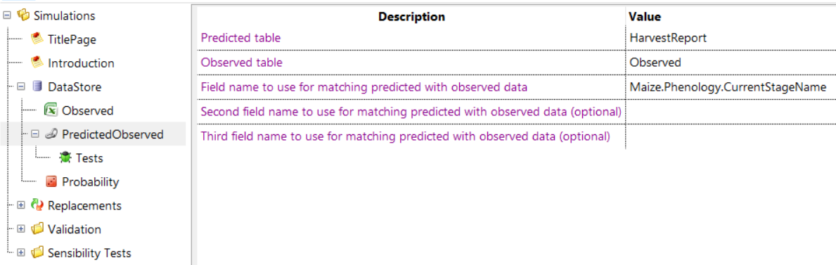
You then specify the name of your predicted and observed tables and the column name you want to match rows on. In the example above, the user interface will iterate through all rows in your observed and predicted tables and look at the value in the ‘Maize.Phenology.CurrentStageName’ column. Where one row in the observed table matches (has the same ‘Maize.Phenology.CurrentStageName’ value) one row in the predicted table, that row will be added to the new ‘PredictedObserved’ table.
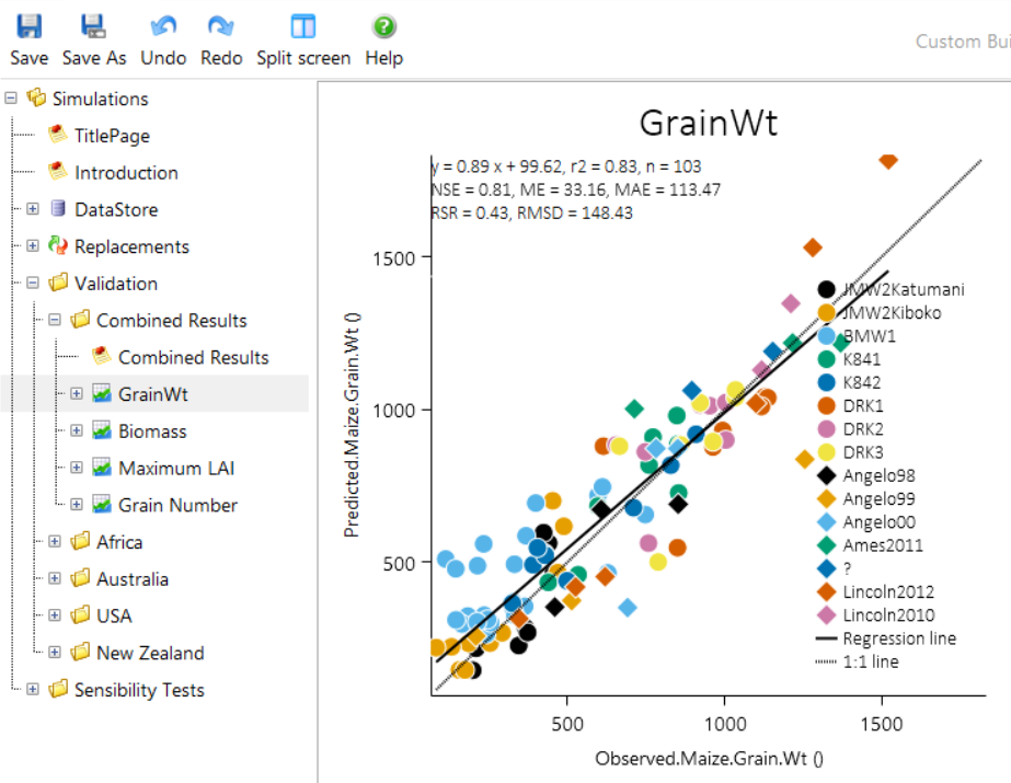
This table then makes it easy to create predicted vs observed graphs.
Testing
Everytime a change is made to APSIM and a pull request is made, Jenkins automatically runs all simulations and ensures that the model validations are still valid. It does this by looking for Tests components under PredictedObserved components. These Tests components calculate a range of statistics and store the ‘accepted’ values of these statistics. When Jenkins runs the simulations, it recalculates the statistics and checks to see if they are different (within 10% tolerance) of the ‘accepted’ statistics. Once a model is validated, a Tests component should be added to the .apsimx file under the PredictedObserved component.
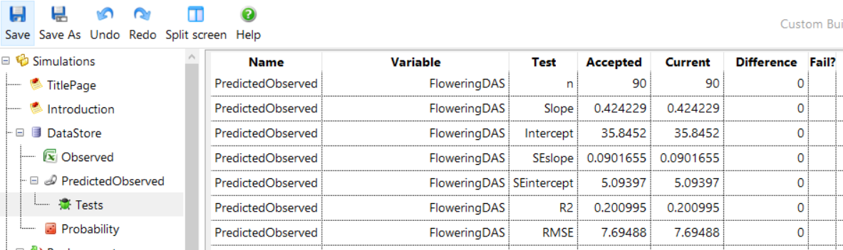
If you need to update the ‘accepted’ values, because for example you have modified the science in the model, you can right click on the Tests component and click Accept Tests. There after the current statistics will be the new accepted ones.
The statistics are:
| Test Name | Description |
|---|---|
| n | The number of PO pairs for the given variable. |
| Slope | The slope of the straight line linear regression. A perfect fit would have a value of 1. |
| Intercept | The intercept of the straight line linear regression. A perfect fit would have a value of 0. |
| SEslope | Standard error in the slope. |
| SEintercept | Standard error in the intercept. |
| R2 | R2 value. Between 0 and 1 where 1 is a perfect fit and 0 is basically random noise. |
| RMSE | Root Mean Squared Error. 0 is a perfect fit. Values less than half the standard deviation of the observed data are acceptable. |
| NSE | Nash-Sutcliffe Efficiency. Indicates how well the PO data fits the 1:1 line. Ranges from -∞ to 1 with 1 being the optimal value while values between 0 and 1 are generally viewed as acceptable. Values < 0 indicate unacceptable model performance. |
| ME | Mean Error between predicted and observed values. 0 is a perfect fit. |
| MAE | Mean Absolute Error. 0 is a perfect fit. Values less than half the standard deviation of the observed data are acceptable. |
| RSR | RMSE-observations Standard Deviation Ratio. The ratio of RMSE to standard deviation. 0 is a perfect fit. |